This post explores where to expect efficiency gains when using the new dtplyr to import and manipulate large flat files.
# Install packages if you need to
install.packages(c("tidyverse", "fs"))

library(data.table)
library(dtplyr)
library(tidyverse)
library(microbenchmark)
Problem
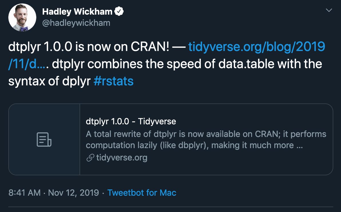
This week, we got the following exciting announcement from Hadley Wickham regarding a big dtplyr release!
When dealing with large flat files, I have often resorted to datatable’s fread function, which is a very fast alternative to readr’s read_csv (for example). Unfortunately, I’m not too comfortable with datatable syntax for data munging, so I have a few ugly pipelines laying around where I mash data from fread into some tibble-ish format that accepts dplyr verbs. In this setting, dtplyr feels like the idyllic solution but, being a lesser mortal than Hadley, I’ve had trouble connecting all the dots.
Specific questions:
- Does dtplyr let me avoid
freadaltogether? (Spoiler: Not really, that’s not dtplyr’s purpose.) - If not, does the main dtplyr function
lazy_dtstill give me efficiency gains when I’ve loaded something fromfread? (Spoiler: Absolutely, that is the point.) - Does
lazy_dthelp when I’ve loaded something fully into memory viareadr? (Spoiler: No.)
Example Data
To illustrate, we’ll use a modest 150MB csv dataset provided by the Gun Violence Archive and available in Kaggle which reports over 260k gun violence incidents in the US between 2013 and 2018. Note that we don’t directly repost the data here in accordance with use agreements; if you’d like to reproduce the below, please download the csv via the above link and stuff it into your working directory.
All we’ll do below is simply load the data, then group by state and print a sorted count of incidents. For each strategy, we’ll keep track of compute time.
Benchmarks
Using read_csv
Here’s the traditional strategy: use read_csv to load the data, and do the usual group_by() %>% count() work.
microbenchmark(
   read_csv("gun-violence-data_01-2013_03-2018.csv", progress = FALSE) %>%
      group_by(state) %>%
      count(sort = TRUE) %>%
      print(),
   times = 1,
   unit = "s"
)$time/1e9
## # A tibble: 51 x 2
## # Groups: state [51]
## state n
## <chr> <int>
## 1 Illinois 17556
## 2 California 16306
## 3 Florida 15029
## 4 Texas 13577
## 5 Ohio 10244
## 6 New York 9712
## 7 Pennsylvania 8929
## 8 Georgia 8925
## 9 North Carolina 8739
## 10 Louisiana 8103
## # … with 41 more rows## [1] 3.373726Using fread
Here’s the same result, but loading with fread. The cool part here, brought to us by dtplyr, is that we don’t have to bring the large data table into memory to use the group_by() %>% count() verbs; we simply cast to lazy_dt and then as_tibble the much smaller results table for printing.
microbenchmark(
   fread("gun-violence-data_01-2013_03-2018.csv") %>%
      lazy_dt() %>%
      group_by(state) %>%
      count(sort = TRUE) %>%
      as_tibble() %>%
      print(),
   times = 1,
   unit = "s"
)$time/1e9
## # A tibble: 51 x 2
## state n
## <chr> <int>
## 1 Illinois 17556
## 2 California 16306
## 3 Florida 15029
## 4 Texas 13577
## 5 Ohio 10244
## 6 New York 9712
## 7 Pennsylvania 8929
## 8 Georgia 8925
## 9 North Carolina 8739
## 10 Louisiana 8103
## # … with 41 more rows## [1] 1.161118This method is about twice as fast!!!
What about objects already in memory?
Maybe the above performance gain isn’t that surprising: a lot of the above boost is likely due to speed improvements with fread, which we already knew about. Does lazy_dt() still save us time when data are already in memory?
Here, we load with read_csv and store as the tibble dat_readr. Then, we do the group_by() %>% count() 100 times.
dat_readr <- read_csv("gun-violence-data_01-2013_03-2018.csv", progress = FALSE)
microbenchmark(
   dat_readr %>%
      group_by(state) %>%
      count(sort = TRUE),
   times = 100
)
## Unit: milliseconds
## expr min lq
## dat_readr %>% group_by(state) %>% count(sort = TRUE) 9.454512 10.20473
## mean median uq max neval
## 11.15166 10.52119 11.14279 53.51589 100Here, we use the same dat_readr object, but cast it to lazy_dt before doing the group_by() %>% count() 100 times.
microbenchmark(
   dat_readr %>%
      lazy_dt() %>%
      group_by(state) %>%
      count(sort = TRUE),
   times = 100
)
## Unit: milliseconds
## expr min
## dat_readr %>% lazy_dt() %>% group_by(state) %>% count(sort = TRUE) 10.64056
## lq mean median uq max neval
## 11.99145 49.00027 14.5085 83.51196 243.6867 100This second approach is actually slower, which totally made sense to me once I saw the answer! Why would taking extra steps to lazily evaluate something already in memory be faster? Doh!
For completeness, here’s the same example where we store an object dat_dt using fread.
dat_dt <- fread("gun-violence-data_01-2013_03-2018.csv")
microbenchmark(
   dat_dt %>%
      lazy_dt() %>%
      group_by(state) %>%
      count(sort = TRUE) %>%
      as_tibble(),
   times = 100
)
## Unit: milliseconds
## expr
## dat_dt %>% lazy_dt() %>% group_by(state) %>% count(sort = TRUE) %>% as_tibble()
## min lq mean median uq max neval
## 3.85039 4.322646 5.870348 4.492541 4.892027 63.86446 100That’s at least 3 times faster! Word.